
Sh2-220
Sh2-220 - Click here for full resolution
Sh2-220, also called NGC1499 or the California Nebula, is an emission nebula located in the constellation Perseus. Its name comes from its resemblance to the outline of the US State of California in long exposure photographs. It is almost 2.5° long on the sky and, because of its very low surface brightness, it is extremely difficult to observe visually. It can be observed with a Hα filter (isolates the Hα line at 656 nm) or Hβ filter (isolates the Hβ line at 486 nm) in a rich-field telescope under dark skies. It lies at a distance of about 1,000 light years from Earth. Its fluorescence is due to excitation of the Hβ line in the nebula by the nearby prodigiously energetic O7 star, Xi Persei, also known as Menkib, seen here as the bright star at the bottom of the image.
source: Wikipedia
NGC/IC:
Other Names:
Object:
Constellation:
R.A.:
Dec:
Transit date:
Transit Alt:
NGC1499
California Nebula, Sh2-220
Emission Nebula
Perseus
04h 02m 12s
+36º 40’ 53.8”
30 November
73º S
Conditions
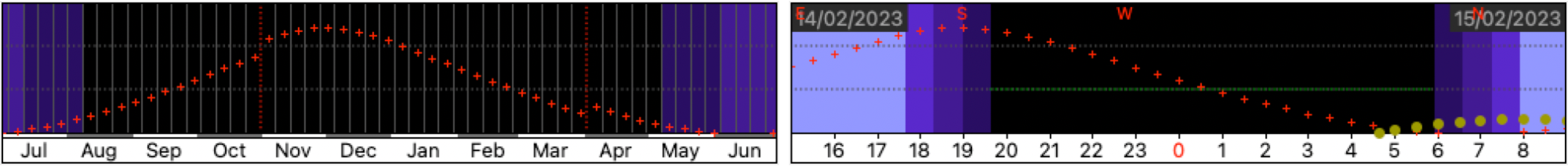
While technically a circumpolar object, NGC1499 can best be considered a winter object, with optimal visibility from October until February. Subs were taken on five nights between 07-14 February 2023. During the early parts of those nights, the object was high above the horizon and could be photographed until just after 01:00h at night. The moon was rising later in the evening during the first sessions, and fully absent during the later sessions. Weather conditions were a bit hit and miss. Humidity was mostly high between 85 and 95% and during several parts of the sessions too much clouds prevented from imaging. So from the 6 hours or so imaging window in each of the nights, several hours were lost due to weather conditions. Temperatures were ok and fluctuated around the freezing point.
Equipment
The Takahashi FSQ-106 was used for this image in its standard configuration and paired to the ASI6200MM full frame camera. Due to the fluctuating weather conditions the equipment was not left outside between all five imaging sessions. For some sessions even, the decision to setup and image was made well into the evening. The new setup with rolling pier proved itself extremely efficient and allowed very short setup times. A drawback of these last minute decisions however, is that the telescope is still acclimating to the cold outside temperatures during imaging. The shift in focus during that first 1-2h of imaging is quite significant. And while I did refocus fairly regularly, still some frames had to be thrown out due to poor focus. During this period I was testing out different flat panels. The result is that the RGB images were calibrated using the Aurora flatpanel, while the SHO images were calibrated using the Flatmaster panel. For the Aurora I had to modify exposure times to get to a target ADU, whereas for the Flatmaster, which brightness can be adjusted in software, all frames could be taken at 5s. This meant a lot more calibration frames when using the Aurora.
Telescope
Mount
Camera
Filters
Guiding
Accessoires
Software
Takahashi FSQ-106, Sesto Senso 2
10Micron GM1000HPS, EuroEMC S130 pier
ZWO ASI6200MM Pro, cooled to -15 ºC
Chroma 2” LRGB unmounted, ZWO EFW 7-position
Unguided
Fitlet2, Linux Mint 20.04, Pegasus Ultimate Powerbox v2, Aurora Flatfield, Pegasus Astro Flatmaster 150MBox
KStars/Ekos 3.6.2, INDI Library 1.9.9, Mountwizzard4 3.0.0, PixInsight 1.8.9-1
Imaging
Narrowband imaging with these 3nm filters and the FSQ-106 is usually done using 300s (5 min) exposures at Gain 100. However, to speed up the focusing routine, many of the focus frames were taken using gains of 300 or 400. In some instances that wrong gain setting had somehow unintentionally carried over to the imaging sequence. This complicated the calibration efforts quite a bit, requiring extra darks. Together with the calibration complications of the Flat frames (see above), the overall calibration got a bit complex, but nothing that WBPP could not handle.
There are different ways to image NGC1499. It is a great Ha-target, and many astrophotographers show the image in either broadband or Ha mapped to the red channel. In those cases, the nebula comes out as an intense red nebula. However, there is also a very strong SII signal and there is also a fairly significant area that shows a faint OIII signal. So I decided to image in all three channels and process according to the Hubble palette. To bring out the OIII signal was not easy. At my not so dark bottle 5 skies, there is hardly anything visible in a single 5min OIII sub. It is only with stacking that the nebulosity comes out. So I decided to capture a lot of OIII and ended up with ultimately almost 8h of OIII data. The exposure of other channels was almost matched. To make sure the stars would have their natural colors, a small set of broadband RGB data was acquired. In total this led to a pretty long overall exposure for my setup of almost 22h.
The target is very large and only barely fits within the 3.5º Field of View. Therefore precise framing is important. When doing a regular GoTo command with the software, the target did not really fit very well in the frame. So a manual adjustment was made to the positioning, and a reference image was saved to position in exactly the same way in subsequent sessions.
Resolution
Focal length
Pixel size
Resolution
Field of View
Rotation
Image center
9576 × 6388 px (61.2 MP)
530 mm @ f/5.0
3.76 µm
1.460 arcsec/px
3º 53’ x 2º 35’
44.7 degrees
RA: 04º 00’ 47.798”
Dec: +36º 35’ 53.72”
Processing
All frames were calibrated with Dark (50), Flat (25) and Flat-Dark (50) frames, registered and integrated using the WeightedBatchPreprocessing script. At the time of taking these images, some experiments were conducted around making Flat frames. As a consequence, Flats were taken with two different Flat panels, one of which did not allow brightness control. So for that panel exposure time was used to get to the target ADU values. Also, some early images were taken at the wrong gain values. Taken together, this resulted in a large variety in exposure times and gain settings, for which all (Flat-)Darks were taken. When putting all of this in WBPP, the complexity of what needed to be calibrated with what was enormous. Nevertheless, WBPP allowed to manage everything in one go. This is a testament for how flexible WBPP is these days. In earlier iterations, such a complex set of calibration combinations would have required multiple runs of the script, each focusing on different images. But now WBPP allows in an easy way very precise targeting of calibration frames to light frames. The early higher gain value narrow band images were combined with the gain 100 images without any problems.
SHO image
NGC1499 is a very bright target in H-alpha. But what was unknown to me was how much signal there was in the SII line. Lots of structure, and in some areas even more detail than in H-alpha. This was so much different for OIII. On individual images there was barely any signal visible, and only after stacking the signal came through.

Stacks of the individual narrowband images for H-alpha (left), OIII (middle) and SII (right).
The narrowband images were processed in a starless mode, so first StarXTerminator (SXT) was applied. There was not much gradient, but the little bit was removed using DynamicBackgroundExtraction. Normally I use a fixed pattern of points, but because there was nebulosity all over the image, the points were now manually placed in areas where it was clear that there was no nebulosity present. The deconvolution with BlurXTerminator (BXT) only had a very subtle effect. On these starless images, BXT cannot make an automatic PSF estimate. So instead, the stars-only images were used to assess the FWHM using the script Scripts/Image Analysis/FWHMEccentricity. The FWHM came out at 2 pixels. In BXT different PSF values around 2 were tested. With higher numbers the effect was a bit more pronounced, but with too high values artefacts started to appear. In the end a value of 2.5 was used. Images were stretched using the GeneralisedHyperbolicStretch function. For any significant contribution, the OIII signal had to be stretched pretty far, which made it very noisy. That’s why initial noise reduction was applied using NoiseXTerminator (NXT) for the OIII only. During stretching an attempt was made to get all three channels to about the same brightness level. However this was not 100% correct, leading to some magenta color cast in the background when combining all three. Therefore a LinearFit was applied to OIII and SII with H-alpha as the reference. The combined SHO image came now out pretty colourful, but with a colour neutral background. The image was very yellow and very bright, and the SHO balancing script from Bill Blanshan did not result in a pleasing overall colour palette. So the traditional method was used of selectively applying color masks and manipulating the colour channels within them. The yellows were pushed down a bit and made more bronze-orange. The greens were toned down a bit and the blues were enhance a tiny bit.
From here on the further processing involved some more subtle enhancements to bring out a bit more contrast and detail. The DarkStructureEnhance script was applied, followed by two rounds of LocalHistogramEqualisation. First the smaller structures were targeted with a kernel radius of 112, followed by an increase in detail in the larger structures with a kernel radius of 300. An attempt to bring out even more detail using BXT was done, but this did not affect much anymore. A few color blips had creeped into the image, which were stamped out using the CloneStamping tool.
RGB Stars
To get a narrowband images with stars in their natural colours, 1h of total exposure in the RGB channels was made. Stacks of the individual colour channels were deconvoluted before putting them together into one RGB image. In my experience this gives better results than combining first and then run BXT. Since only the stars would be used from this image, no DBE was applied. Colours were calibrated using SpectroPhotometricColorCalibration and stretching was done by simple HistogramTransformation. The stars were extracted using SXT. At this point it was a non-linear image, so I could have chosen to unscreen the stars at this stage. Instead I chose to extract the stars as they were. The stars could now be added to the SHO image and in that PixelMath process I used the screening function.
Final Image
The image was now almost ready. As finishing touch a mild noise reduction (amount 0.5) was applied. Also this is typically the time when a few rounds of small adjustments using CurvesTransformation is typically applied. In this case some very small colour casts in the background were reduced. And overall the image was flattened a tiny bit. After applying the various tools to bring out detail, overall the image looked a bit too contrasty, so this was reduced using an inverse S-curve.
Processing workflow (click to enlarge)
This image has been published on Astrobin.