
ASI533MM Pro - First Impressions
A camera that has received a lot of positive feedback in the last few years, was the ZWO ASI533MC Pro. Recently Sony released the mono version of the IMX533 sensor in this camera. This sensor has now made its way into astrocameras. Both QHY (QHY533m) and ZWO (ASI533MM Pro) have developed a camera based on this sensor.
Market Positioning
ZWO markets this camera as a beginner camera and tends to compare it to the popular ASI183MM Pro. However, for my purposes, the camera will be used as a replacement for the even more popular ASI1600MM Pro. The ASI1600 has been a fantastic workhorse over the last five years, but the Panasonic MN34230 micro four-thirds sensor is really showing its age when compared to newer sensors. For example, the ASI6200MM Pro that was purchased 1.5 years ago, is so much better. Of course it has a much bigger sensor, but apart from size, it really blows the ASI1600 away in terms of noise performance, dynamic range, amp-glow, sensitivity, etc. The ASI533 promises to be all that modern-sensor performance, in a much smaller (and cheaper) package.
Getting the camera
On the day the camera was announced, the order was placed directly with ZWO in China. Direct ordering from ZWO has worked very well in the past and now was no exception. The order was placed on April 6, and showed status ‘backordered’ with estimated delivery time May. On May 30, the package arrived in the post. In the box no surprises for anyone that is familiar with the ZWO cameras. A set of spacers and adapters in M42/M48 sizes, USB cables and a nice padded case accompanied the camera itself.
Size
The sensor of the ASI533 measures 11.3 x 11.3 mm. That is a bit smaller than the 17.7 x 13.4 mm of the ASI1600. But for the galaxies and star clusters that the ASI1600 was typically used for, sensor size was not a limiting factor. Larger nebulae are shot with the ASI6200. The benefit of the small-sized sensor is that it is a perfect fit for the 1.25” mounted Astrodon filters that were used with the ASI1600. Replacing the ASI1600 with a bigger camera, for example the ASI2600MM Pro, would have meant a whole new set of filters.
For the connection with the filter-wheel, the ASI533 is also a simple swap with the ASI1600. It comes with the same M42 male threaded connection that screws right into the EFW. And the back focus distance is also the same at 6.5mm.
A big difference, and subject to some debate, is that it’s a square sensor. Some love it, some hate it. Personally I belong to the first category. Many targets have a round shape, and compose very well in a square geometry. And if you really want a rectangular shape, the 4:5 aspect ratio is a very common one used in photography and would require only a marginal crop.
Size was also the reason to go with the ASI533 and not with its QHY counterpart. The QHY is much bigger and almost twice as heavy. Also the backfocus distance is different, so it would probably have meant a bit more than just swapping out the ASI1600.
The Field of View of the Takahashi TOA-130 telescope (1000mm) with both camera’s. The slightly smaller sensor of the ASI5333 as compared to the ASI1600 is not a problem for many objects.
Specifications
The sensor of the ASI533 is a backside-illuminated sensor, which is equivalent to a low-noise sensor. The digital information is read out from the sensor in 14-bit format. This is less than the 16 bit of the ASI6200, but a significant step up from the 12 bit of the ASI1600. Like many modern sensors, it has a dual-gain architecture. This means that at a certain gain setting (in this case: 100), different circuitry comes into play, resulting in a massive drop in noise and increase in dynamic range. Unless you’re dealing with very high contrast images, setting the camera at this gain of 100 is probably the most effective for most situations.
Sensor: Sony-IMX533CLK-D; 3008 x 3008 pixels; 9MP
Dimensions: 11.31 x 11.31mm; 15.968mm diagonal
Pixels: 3.76 µm, 50000e full well capacity
Dimensions: 78mm diameter, 470g

The square sensor format may not be everybody’s favourite aspect ratio, but allows framing galaxies and clusters very well.
Getting started
Installing the camera was pretty easy, as it uses the same connections and dimensions as the ASI1600. Getting the camera recognized by the software (KStars/Ekos) required an update of the software. In my case I upgraded from KStars 3.5.7 to 3.5.9, which includes the latest INDI drivers (version 1.9.6). Clearly software that runs the ASI533MC Pro does not work automatically with the ASI533MM Pro. Other users have reported similar driver upgrade requirements for ASCOM.
Once connected, there are very few INDI settings to worry about. Gain and offset (see below) are the most important ones. The ASI6200 has an on-sensor dew-heater installed that can be turned on or off, but this seems to be lacking with the ASI533. The small sensor probably wont need it.
The 9 Megapixel files from the ASI533 download as 18MB Fits files. When you’re used to the massive 62MB Fits files from the ASI6200, or even the 32MB Fits files from the ASI1600, these much smaller files really make the whole workflow a lot quicker.

The dual-gain nature of the sensor shows a sudden drop in noise levels at Gain 100, while increasing the dynamic range to almost the maximum level of Gain 0.
Gain and offset
As mentioned above, there are basically two gain settings to use. Gain 0 to benefit from maximum full well depth for very contrast-rich objects. And Gain 100, the gain at which the noise suddenly drops and dynamic range increases. Increasing the gain higher than 100 has no benefit. The reduction in noise is almost negligible, while full well depth and dynamic range drastically reduce. So Gain 100 is typically a ‘set and forget’ setting.
Offset is a bit more difficult to assess. There is no information in the camera’s documentation. The source that many people rely on is the default setting in the various drivers. When reading on-line sources, offset values somewhere between 10 and 70 are reported. How can we take a better calculated approach to this?
Offset is a default value that is added to each pixel’s readout. The main purpose is to ensure that this readout is always bigger than 0. Any value lower than 0 would miss information, but more importantly, during processing, algorhythms can behave very weirdly if they have to deal with 0 numbers. So the offset should be high enough so that every pixel has a value.
Similarly Offset should not be unnecessarily high. A too high offset just shifts the histogram to the right, reducing the total usable width, with no benefits. A proper offset can be easily assessed by taking a series of dark images.
To determine the minimally required offset, dark images of 60 seconds were recorded using increasing offset values. For each image, the image Statistics tool in PixInsight was used to measure the Mean and Minimum pixel values. This was repeated for both gain 0 and gain 100. The results are plotted in the graph below.
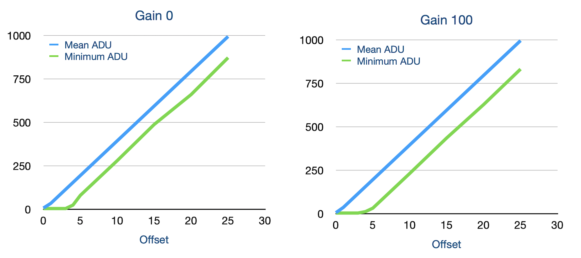
At low offsets, the value of some pixels is cut-off to 4. With an offset of 5 for both Gain 0 and Gain 100, the true signal of every single pixel is measured as a realistic ADU value.
Interestingly, even with offset 0, the minimum value was still 4. As this is the converted value from 14-bit to 16-bit, the minimum sensor readout must have been 1. This raises the question if we should be worried about 0 values at all? Or have camera manufacturers already taken care of it, and sensors never show a value of 0? However, as can be seen from the graphs, at the lowest offset values the value of 4 actually represents a signal much lower than 4, so not representative for the value measured. But at offset 5, the curve lifts off the floor and minimum/mean ADU values follow each other proportional to the offset value. At gain 0 this happens a fraction sooner, but the difference is not much. Offset 5 seems to be the right setting for both gain 0 and gain 100, to ensure that also the lowest possible signals are measured properly.
Also, the graph shows that one unit of offset equals 40 ADU. So by adding an offset of 5, the increase in ADU values is 5 x 40 = 200. This is negligible compared to the 65,536 maximum ADU value. On the other hand, if you use an offset of 70, this equates to an increase in ADU values of 70 * 40 = 2800. Still much smaller than the 65,536 maximum value, but not totally negligible anymore.
Darks and Bias
The camera was cooled to -15 ºC. For my climate I’ve made this temperature setting a kind of a standard. It can be used in ambient temperatures between -15 and 20 ºC. Hardly ever are the conditions outside of those limits. With Gain 0 and 100, both using an offset of 5, a library of darks and biases was built. Inspecting these results gave some nice insights into the performance of the camera.
First of all, like advertised and in line with other modern cameras, there is no sign at all of amp glow. The dark frames look nice, even and clean, even up to 5 minutes. The only visible effect of longer dark exposures is the more prominent appearance of ‘warmer’ pixels. In a stretched dark, these look like worrying white pixels. But when you look at the ADU values of these ‘white’ pixels, they are only 50% or so brighter than the dark background. Something that will easily calibrate out, or better still, average out when using dithering.
Interestingly, the mean ADU values of the dark and bias frames were almost identical. If you subtract a bias from a dark frame, you end up with lots of 0 values. And this is the same whether you take a 30s dark or a 300s dark. The only difference between the short and long dark frames are the ‘warm’ pixels (see image). This means that the dark current is pretty much absent, and one could really wonder if bias frames for calibration are needed at all.
In contrast, these results can be compared to the ASI1600. Here prolonged dark exposures lead to much higher overall noise levels, due to dark current. And in addition, in the longer dark exposures the amp glow starts to appear.
The background signal is very similar between short and long darks (all stretched with same STF-settings). The main difference is the appearance of somewhat ‘warmer’ pixels at longer dark exposures. In contrast to the ASI1600, which dark current leads to much brighter background levels and multiple areas of amp glow in longer dark exposures.
Calibration strategy
The extremely clean dark and bias images coming from this camera may prompt a revisiting of the calibration strategy. To calibrate light frames, the use of bias frames has limited additional value. Just an exposure/gain/offset matched dark would be more than sufficient. One might even think that with proper dithering, dark frame calibration may not be as crucial as it used to be.
Something similar may be true for flat frames. Still it would probably remain good practise to subtract either a bias frame or a time-matched dark frame (flat-dark) before using the flats in further calibration.
It would be interesting to do some further experimenting with actual use of the camera and see if and how traditional calibration strategies could be simplified using cameras with such a low noise level and clean signal.
Lights
With the camera just having arrived yesterday, and in absence of any astronomical night at the moment, there has been no opportunity yet to test the camera out in real life. I will leave this for a future post. Aaron from Alaskan Astro has been using the QHY533m as a beta-tester for a while and made a direct comparison with the ASI1600. As you can see at 10:10 minutes, the differences in dynamic range, full well depth, bit-depth, etc. lead to an image with a lot more detail and contrast. Granted, this is the QHY version, but the ZWO version would probably see similar results.
Conclusion
It is too early to draw a full conclusion on the camera. For that, actual images need to be taken, examined and compared. But the first impression is that this camera is in every aspect a massive upgrade compared to the ASI1600. Absence of any dark current and amp glow, very even and clean noise-pattern and at most a random pattern of somewhat ‘warmer’ pixels that can be easily calibrated out, make this a very solid performer.
In my use-case, alongside the bigger ASI6200, the upgrade from the workhorse ASI1600MM Pro to the somewhat smaller, but much more modern ASI533MM Pro seems to be working out well. The 7 Astrodon broadband and narrowband filters will enter into their second career in front of this new addition to the observatory.