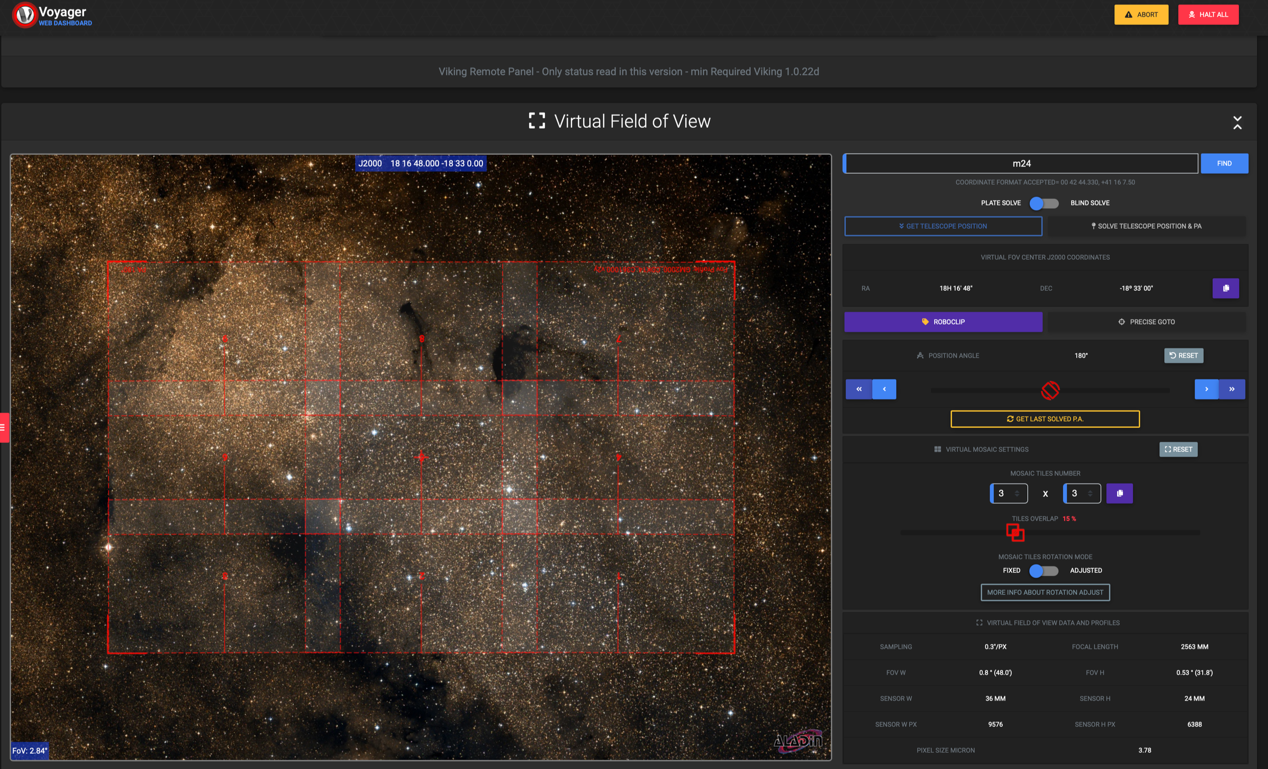
A 3×3 panel mosaic was the only way I could capture M24 using my long focal length setup in the remote observatory. Voyager Advanced Software was very helpful in defining the required panels with their coordinates.

If a target is too big for the Field of View of your telescope/camera combination, a common solution is to make a mosaic. Multiple partially overlapping images are stitched together to make one much bigger image. One of the last objects of the Messier catalogue that still needed photographing was M24, or the small Sagittarius star cloud. At roughly 2°x1°, this is a pretty large target, just slightly smaller than the Andromeda galaxy. For my main telescope in Spain, with a Field of view of about 48’x32’, this target is much too big. My wide field setup in the backyard could be used, but M24 has a declination of -18°, making it difficult to photograph at a northern latitude. Adding to the complexity is that this is a summer target, when nights are short at home. In early fall, M24 is just visible for perhaps 2-3 hours after sunset, at very low altitudes of around 10°. My backyard does not even have access to that sky, so it would mean going out to a dark site with low horizon.

So the choice was to either make my first mosaic with my main setup, or hope for a few very clear nights in early fall and grab 2-3h of exposure with my wide field setup. I chose the former. This would be a great opportunity to practice making mosaics, something I’ve always wanted to try out.

Planning

In planning a mosaic, some kind of virtual Field of View option is crucial. KStars has this built in and can output straight to the scheduler. In Voyager Advanced, the web dashboard contains such a mosaic view in the virtual Field of View tool as well. When pulling up M24, it was hard to determine where M24 started and ended. It is just a massive star-field. With some research I was able to get a good idea of the required field of view. And while the original plan was a 2x2 or 2x3 mosaic, assuming 15% overlaps, it was clear that this had to be a 3x3 mosaic. That meant 9 panels! That is a lot of images to shoot and process.

M24 is essentially a star field and exposure does not have to be long. For 9 panels I chose eventually 5 hours exposure per panel, using only RGB filters and no luminance. This is a little bit shorter than most my globular clusters, which generally come out well. With nine panels though, it would still mean 45 hours of exposure.

Unfortunately Voyager only partly supports the capturing a mosaic. The 9 panel grid from the virtual Field of View can be exported as a target into Roboclip. But a mosaic target in Roboclip cannot be used in Target Manager. The alternative Voyager offers is a tool called Research & Survey, but this does not run in automatic mode. The solution is to export a list of coordinates for each of the panels and manually enter them as individual targets in Target manager. So that is what I did. I also added manually a panel number to each object name to ensure that downstream during processing the files can be identified and processed properly.

The full-frame sensor in the camera is 60MP. So a 9 panel mosaic would create a massive image with a whopping 500MP resolution. Add to that the storage requirements and processing resources and it was quickly realised that this was a situation where binning would be the right thing to do. In bin 2x2 the resulting file would still be over 100MP with a pixel scale of 0.6 arcsec/px. Plenty of resolution and size for the type of object that M24 is.

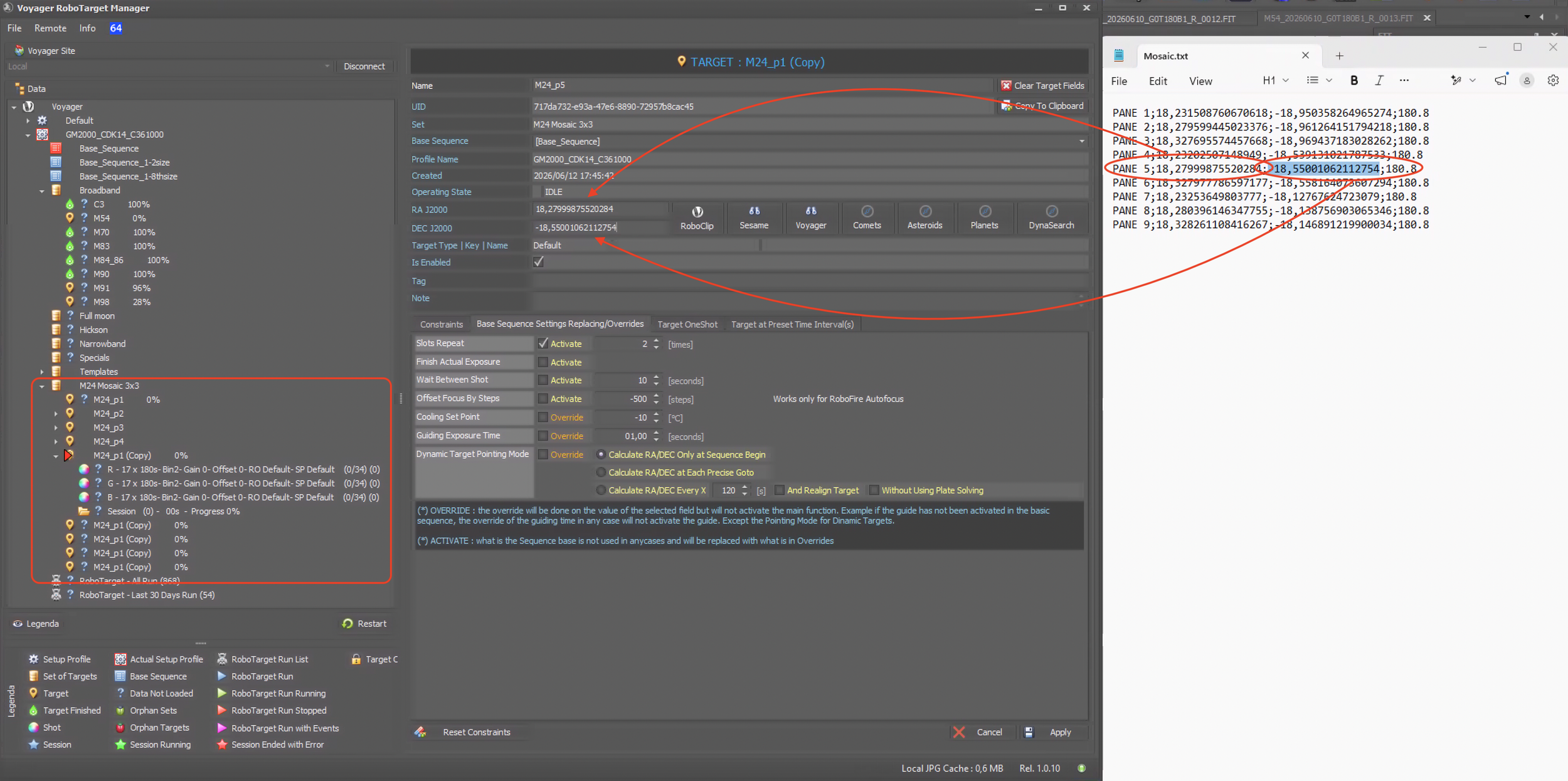
Unfortunately Voyager does not have an option to automatically load the mosaic panels into the Target Manager. But using manual copy/paste a set of 9 targets were created in target manager, ready for automated imaging.

Acquiring data

Once each panel was loaded as a separate target, shooting the images was the same as for every other target. M24 has a declination of -18°, so from the observatory, the maximum altitude was only 33°. Normally I try not to shoot lower than 30°, but in this case that limit was lowered to 20°, leaving a maximum of 6 hours per night to shoot the images. In total it took about a month to capture all required data, from mid June until mid July 2026.

One of the things that I had almost forgotten, were proper calibration frames in Bin 2 mode. Darks need to be collected at the same binning as the light frames, as the noise-pattern that it is correcting for is on pixel-level. For flats is is less critical. Compensation for light fall-off and dust particles can also be done with flats that are binned during post processing. But flats also correct for pixel response non-uniformity (PRNU), and that is a correction on the pixel level. So In the end I decided to make a fresh set of dark and flat calibration frames at bin 2x2.

Processing

There are many approaches to processing a mosaic. And a lot comes down to the order in which you do things. It may be tempting to just process each panel to a near-finished image and use conventional stitching software such as PTGUI to put it all together. However, even the smallest differences between panels in their processing may result in seems between panels that are hard to get rid of.

Generally much higher quality results can be obtained by stitching the panels early in the processing, during the linear stage and before combining the colour channels. PixInsight has a whole suite of great tools to support such a workflow and that is what was applied here. Not all come standard in PixInsight, so be sure to load them all by adding the following repository: https://pixinsight.astroprocessing.com/ . The scripts are developed by John Murphy and can be found under Scripts\>Mosaic.

The processing approach can be divided into the four phases: Preparation, Alignment, Stitching and Processing

Preparation

This includes the normal steps of preparation for every image. Remove stacking artefacts and background gradients. Automatic tools such as GraXpert work well here. Typically this is not the phase where a full deconvolution takes place, but it is generally advised to run BlurXTerminator in ‘correct only’ mode at this stage.

Alignment

Then the images need to be aligned for stitching. The tool used for that is MosaicByCoordinates. As the name implies, it needs to know the coordinates of each panel, so the first step is a plate solve for each of the panels. Then the panels are fed into the tool and the script creates a big black canvas big enough to contain all images. For each panel it produces an output file with the dimensions of that canvas, with super-imposed the panel at exactly the right spot.

An alternative is to create an artificial star field using the CatalogStarGenerator script in PixInsight. Then you can align all images to that artificial field as reference. The output is very similar, a big black canvas with superimposed the image panel. But it requires an extra step and MosaicByCoordinates is easier.

*The MosaicByCoordinates script creates a large black canvas and creates an output file for each panel the size of that canvas with the panel superimposed.*

Stitching

The tool for stitching the panels is PhotometricMosaic (PMM). PMM assumes hard edges on each of the panels. If that has been taken care of in an earlier step, for example using DynamicCrop, additional trimming may not be necessary. But if there are some frayed edges, there is a dedicated mosaic tool that can take care of that. It is called TrimMosaicTile. For each edge the number of trimmed pixels can be set individually. Once the panels have hard edges, the next step is to put all panels together using PMM.

PMM makes two kind of corrections before stitching. It applies a scale factor and a surface spline. The scale factor is determined by stellar photometry and ensures the same stars have equal brightness in the overlapping areas in both images. The surface spline looks at the relative gradient between the two images in the area of overlap and corrects for any differences. By correcting stars and background gradients independently, optimal overlap between panels can be achieved.

PMM can only stitch two panels at a time, one is the reference view and one is the target view. So for larger mosaics, rows or columns need to be built first panel by panel and then the rows or columns need to be stitched. In my 3x3 mosaic I started building each row into a 1x3 mosaic. Then the rows were stitched together one by one to create the final 3x3 mosaic.

The PMM tool has many parameters to set, but most of the time the default settings work well. The main parameter to choose is the Combination Mode. I used Overlay successfully, but some suggest Blend or Average are better options. So feel free to experiment with them and judge the results. In the output files a mask is created to show the seem lines of the overlapping area, and there is a separate ‘overlap’ view added to the file, in whihc the stitching quality can be reviewed in great detail.

With the availability of PMM there is no real reason to use alternative techniques. But if you’re in for some experimenting, other tools have been used with good success as well. One of these tools for example is DNALinearFit from TrappedPhotons.com. It equalises the brightness of the various panels. The stitching can then be done with GradientMergeMosaic (GMM), a default process in PixInsight. Always worth a try, but PMM is the more advanced option, while still very easy to use when most is left in default mode.

PMM only stitches two images at a time. So to build up bigger mosaics you have to start by building up rows or columns. In my case I built up three rows. Once they were completed I used the same process to stitch the rows together, as if they were individual panels.

Processing

Looking back at the big picture, individual mosaics are built per colour channel. So for an RGB image, like I had for M24, the whole process has to be repeated three times. And the result is a set of three large mosaic images that should be processed the same way as any other RGB image. It is advised to check alignment between colour channels. If the procedure is followed as per above, the three mosaics are perfectly aligned. But it is easy to loose track of all the panels, so if something had gone wrong and led to a slight misalignment, now is a good time to correct.

Further processing from here is pretty standard. You probably want to crop the stacking/stitching artefacts away and define the composition cutout of the mosaic. Gradient correction should not be needed at this stage anymore. Instead now is the time to put the RGB image together using ChannelCombination and run deconvolution, for example with BlurXTerminator and colour balance, for example SPCC. Stretching with the tool of choice and fine-tuning brightness, contrast, sharpness and colour saturation typically complete the processing. In my case of M24 I had some difficulties with getting to the right colours, probably a consequence of the super dense star field of this specific image. I had to make some manual adjustments. More details on that on the dedicated M24 page on this website.

Conclusion

When the idea came up of making a mosaic on M24 it felt like it would be a very difficult solution to a relatively simple problem. But then I realised that a ‘stars only’ target might actually be the perfect entry into creating mosaics in astrophotography. And starting with a 9 panel mosaic may not sound like the easiest way into the subject. But it turned out that size mainly adds time and complexity, not so much difficulty. You basically do the same thing just a lot more times. In the end the whole project was easier than I had expected.

The result is a massive image with a whopping 100 Megapixels. Regular screen sizes don’t really do justice to the amount of detail that’s in the image. Therefore, I highly recommend to look at the image in this full resolution version. You can zoom in and scroll around to closely watch all 12778 × 7993 pixels. Sure, at the end it is just a bunch of stars. A highly detailed emission nebula might be a better target for so much resolution. So who knows that might become a next project. In any way, having gone through this, using the mosaic approach is now definitely part of my astrophotographic techniques that can and will be used.

Making a mosaic

Planning

Acquiring data

Processing

Preparation

Alignment

Stitching

Processing

Conclusion

Total Solar Eclipse Spain - The Journey