M24
IC 4715, Small Sagittarius Star Cloud | NGC 6603
128’ x 80’ | 0.6”/px | 12,778 × 7,993 px (102MP)
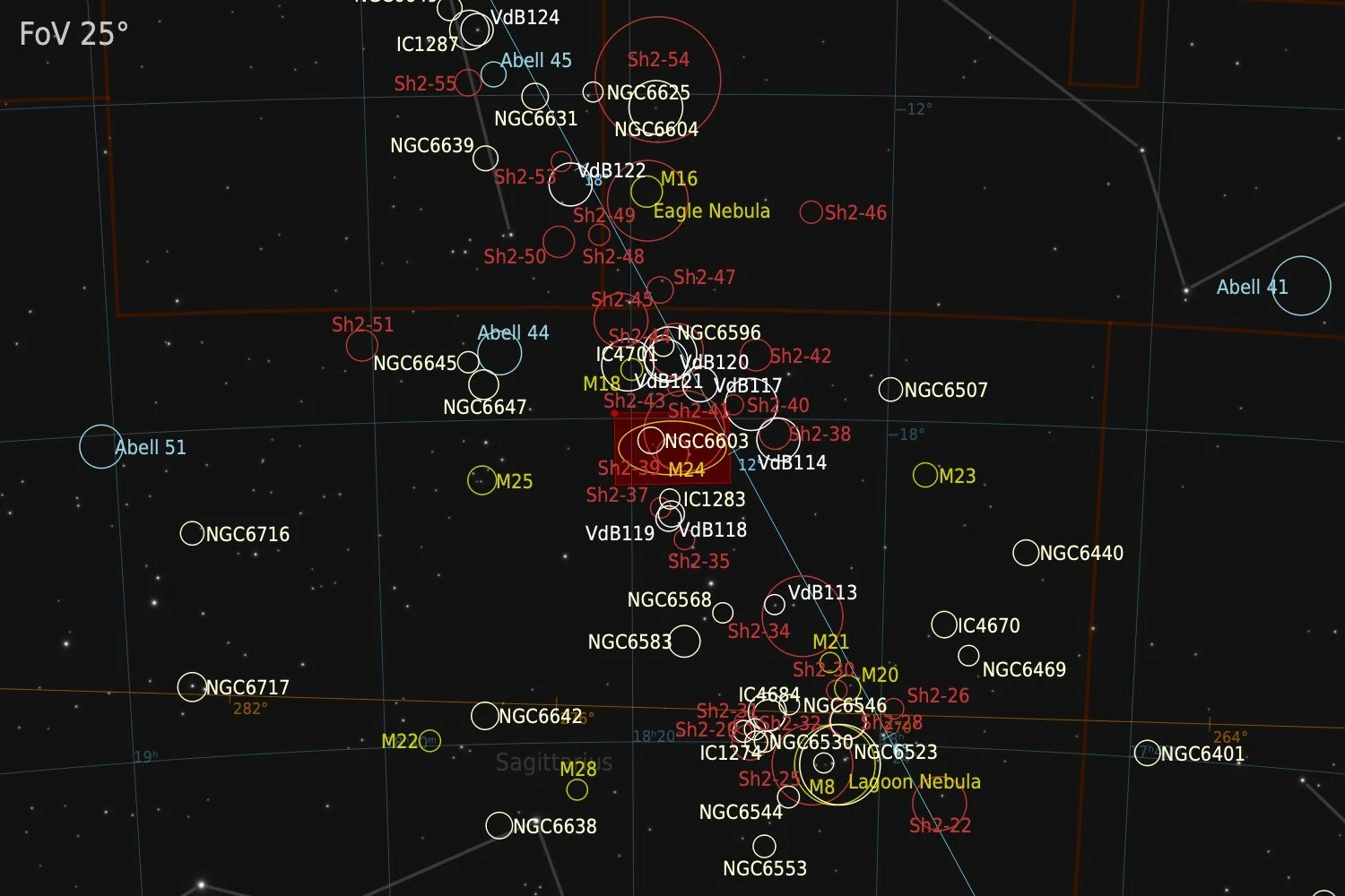
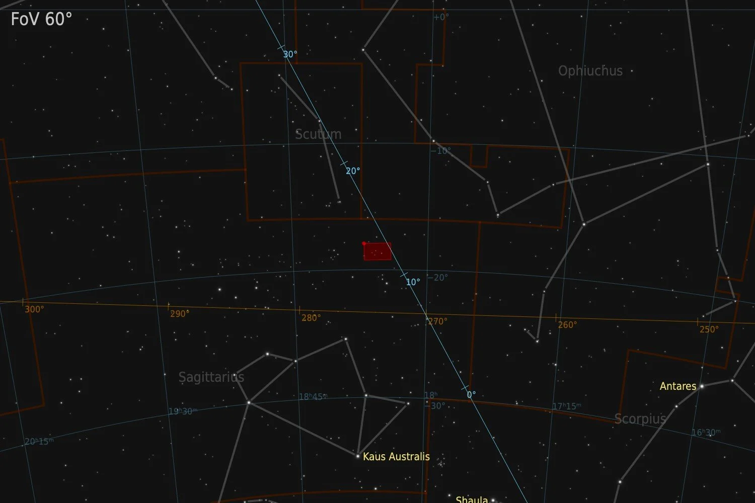
Sagittarius
RA 18h 16m 47s Dec -18° 33’ 05” | 0°
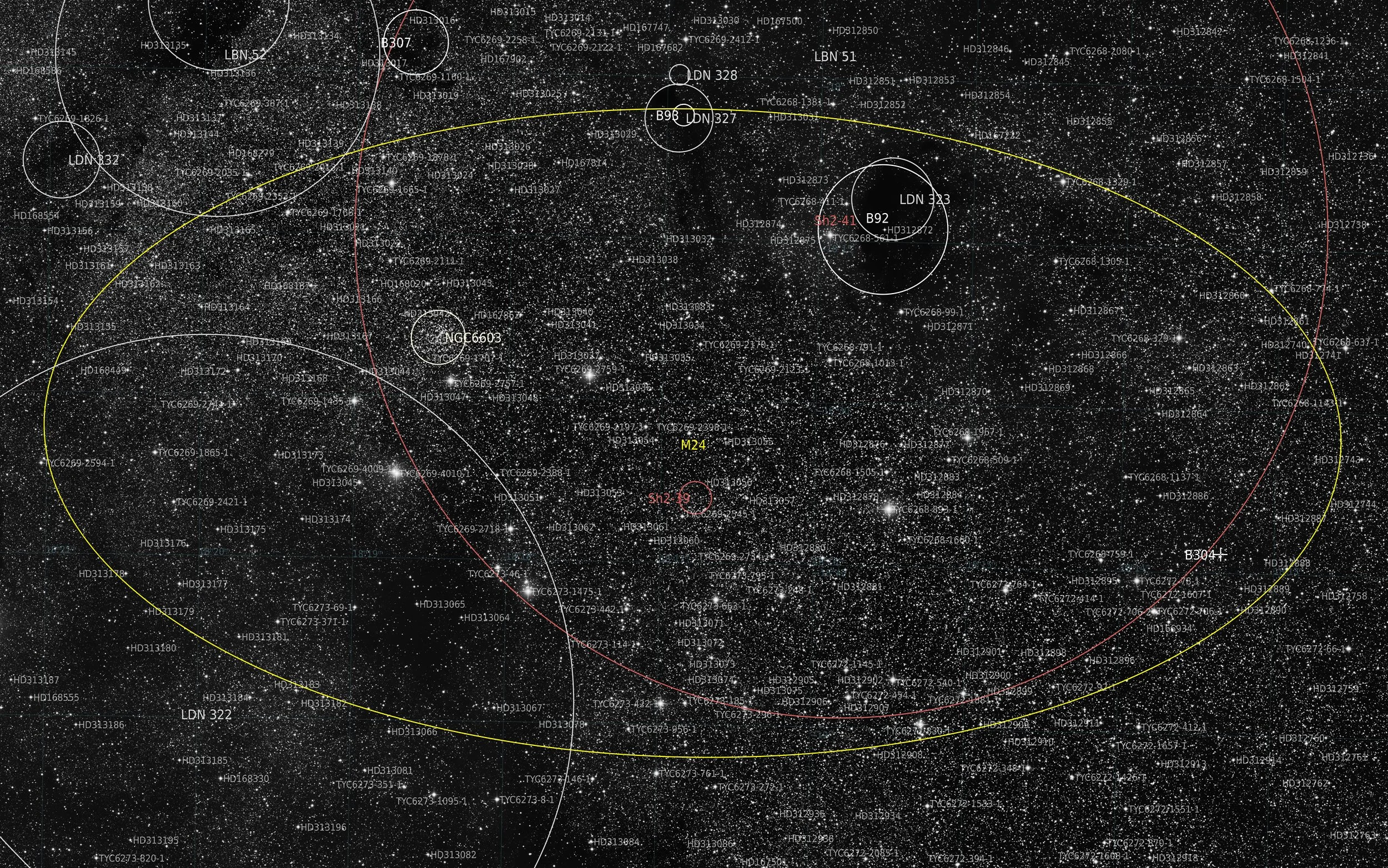
Messier 24, also known as IC 4715, is a star cloud located in the constellation Sagittarius and is commonly known as the Small Sagittarius Star Cloud. It was catalogued by Charles Messier on June 20, 1764, who described it as a large nebulosity containing many stars of different magnitudes. It should not be confused with the Large Sagittarius Star Cloud, which lies roughly ten degrees to the south. The designation IC 4715 arose from a positional error made by Edward Barnard in 1905, which led to the region being added to the Index Catalogue rather than recognised as the same object Messier had originally recorded. M24 is unique among Messier objects in that it is not a deep sky object in the conventional sense — it is not a cluster, nebula, or galaxy, but rather a window through the otherwise dust-laden disc of the Milky Way. Through this gap in the interstellar dust, stars belonging primarily to the Sagittarius Arm of the galaxy become visible at distances ranging from approximately 10,000 to 16,000 light-years, giving the cloud an apparent depth. The cloud itself spans roughly 600 light-years in width and covers an apparent area of around two by one degrees on the sky, making it the largest entry in the Messier catalogue by angular size. Its apparent magnitude of 2.5 makes it easily visible to the naked eye. Within the boundaries of M24 lie several notable objects. The most prominent is NGC 6603, a compact open cluster of around 30 stars discovered by John Herschel on July 15, 1830, situated in the brightest part of the star cloud. Two prominent dark nebulae, Barnard 92 and Barnard 93, are also visible within the cloud as conspicuous voids against the dense star field, catalogued by Edward Emerson Barnard in the early 20th century.
Source: Claude.ai
Data Acquisition
Data was collected during 16 nights in June and July 2026, using a 14” reflector telescope with full-frame camera at the remote observatory in Spain. The object is much too large for this telescope, and therefore the image is shot as a 3×3 panel mosaic. This resulted in a very high resolution. Even in bin2 mode, the original image is over 100MP large. Data was gathered using standard RGB filters. Five hours of data was recorded per panel, so for 9 panels, 45 hours of data have been collected. A total of approximately 39 hours of data was combined to create the final image.
Location Remote hosting facility Roboscopes in Fregenal de la Sierra, Spain (38°N 6°W)
Sessions
Frames
Equipment
Telescope
Mount
Camera
Filters
Guiding
Accessoires
Software
Planewave CDK14 (2563mm @ f/7.2), Optec Gemini Rotating focuser
10Micron GM2000HPS, custom pier
Moravian C3-61000 Pro (full frame), cooled to -10 ºC
Chroma 2” RGB unmounted, Moravian filterwheel L, 7-position
Unguided
Compulab Tensor I-22, Dragonfly, Pegasus Ultimate Powerbox v2
Voyager Advanced, Viking, Mountwizzard4, Astroplanner, PixInsight 1.9.4
Processing
All processing was done in Pixsinsight unless stated otherwise. Default features were enhanced using scripts and tools from RC-Astro, SetiAstro, GraXpert, CosmicPhotons and others. Images were calibrated using 50 Darks, 50 Flats, and 50 Flat-Darks, registered and integrated using WeightedBatchPreProcessing (WBPP). The processing workflow diagram below outlines the steps taken to create the final image.
For an overall description of how to make and process mosaics, see this blog that is written based on the experiences with M24. The first step is to prepare the stacked masters for each colour for each panel. This includes a run of BlurXterminator in ‘correct only’ mode. Generally the stars are looking quite good well into the corners, but running BXT this way just tidies up stars just that little bit. Especially the brighter stars are corrected quite nicely.
Each panel is now aligned to a new master-canvas. The size of that master-canvas is determined by the tool MosaicByCoordinates, based on all 9 panels that are loaded in the tool. The output are panels superimposed on that new canvas. Then the panels are stitched together using PhotoMetricMosaic (PMM). If there are some rough edges on the panels, these are first trimmed off using the tool TrimMosaicTile. PMM is sort of a single click tool, as most of the default settings generally work well. One by one the panels were stitched together. First into horizontal rows, and then the rows were stitched together into full mosaics. The seems were completely invisible. The scaling factors and surface splines applied by PMM apparently did their work very well. These steps were repeated for each of the three colour channels, resulting in three mosaics, one for each colour.
When the colours were put together, it was clear that not every panel had been shot with the exact same brightness level. Differences in imaging conditions, in combination with the very low altitude of the object were well to blame for that. So there were still some gradients in the background. And because this is such a nebulous area in the sky I decided to use MultiscaleGradientCorrection so that my data could be referenced against true values.
Colourcalibration appeared to be a challenging task. The selection of the proper background section appeared to be very sensitive. Probably because of the very dense starfield on top of a cloudy background. I even tried the standard ColourCalibration, but I always ended up with slight colour casts in the background, sometimes red, sometimes green, etc. This was corrected during stretching. After the initial stretches, I corrected individual colour channels in such a way that the background peaks of all colours was overlapping. This may have affected star colour a little bit. The red in the stars for example was a bit too yellow. So I corrected that in the CurvesTransformation tool. And as I was fine-tuning the colours, I also enhanced a little bit the blue in some of the bright stars. After all this fine-tuning of the final colours, the BackgroundNeutralization tool that I always use to get a consistent background across my image library, worked well.
This processing was a combination of standard processing approaches with more unique methods to handle a 3×3 mosaic. In this monograph as well as the blog the essence of all steps is written down. The outline below shows a more schematic breakdown of the processing steps applied to the image.
Processing workflow (click to enlarge)
This image has been published on Astrobin.